How We Scaled Our LLM Inference Infrastructure to Serve 100+ Billion Requests a Week

By Christoph Stuber, Machine Learning Engineer, Superhuman, and Myke Troianovskyi, Tech Lead Manager, Superhuman.

A core part of Grammarly is our GEC (Grammatical Error Correction) model, which continuously runs on a user’s writing and provides suggestions to improve its clarity and correctness. Users see these suggestions as red underlines in their document; they can click into them to view details and accept or reject them. 

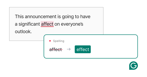
Example of a GEC correction in action 

Unlike most AI features, where a user explicitly triggers a request and waits for a response, GEC is ambient. That makes latency nonnegotiable: Suggestions need to appear instantaneously, or we risk slowing customers down. This presents an interesting challenge for our model-serving infrastructure, which needs to maintain this latency bar at scale—40 million daily active users generating roughly 100 billion LLM requests per week—while remaining resilient to capacity constraints (such as traffic spikes and GPU shortages) and keeping costs in check. 

Our solution is a hybrid architecture that combines internal serving infrastructure with external vendors, layered with targeted optimizations to meet our performance and cost benchmarks. In this post, we trace the evolution of that system and share what we learned for other teams building production-grade LLM infrastructure.

The evolution of our internal GEC infrastructure

Our GEC system started as a pipeline of several small, specialized models (with tens to hundreds of millions of parameters), each built with different techniques and handling different objectives during the correction process. This approach was very flexible, allowing us to scale and optimize each model independently to optimize the overall system. 

Over time, coordinating these different models introduced significant complexity, especially when two models took different approaches to correcting a sentence. For instance, let’s say a user types the sentence “You have an issues.” One model corrects the actual error (by changing issues to issue), while another applies a different solution (removing an in front of issues). We don’t want to naively apply both suggestions, which would result in creating the sentence “You have issue”—which is grammatically incorrect. Therefore, we had to maintain a separate model to decide which suggestion was correct, adding unnecessary overhead. 

We decided to reduce the number of models by using a single, larger, more capable model (1 billion+ parameters). Initially, we were concerned about the serving costs and latency. Larger models require significantly more compute and GPU memory per request, which could reduce throughput per machine. However, in practice, we found that with the right infrastructure and inference optimizations, this approach was cost-competitive (and in some cases, more efficient than the previous system). Here were the optimizations we made: 

1. Using Kubernetes instead of Amazon Elastic Container Service (ECS): Under ECS, our setup was relatively rigid because each service required its own dedicated pool of GPU instances, each with its own instance type. Kubernetes (via Amazon EKS on AWS) gave us more flexibility, allowing us to use different instance types within the same workload (even across instance families). This allowed us to make the most of our existing AWS capacity, especially handy since our new model was more computationally intensive. Fortunately, our broader platform infrastructure team had already laid the groundwork for this switch. 
2. Leveraging vLLM for inference and model serving: We explored several options, including extending our internal inference framework and other open-source options. But none of them matched vLLM’s serving efficiency, which increases throughput by packing more concurrent requests onto existing GPUs with continuous batching. vLLM also supported a wide range of models, giving our team the flexibility to experiment with different architectures.
3. Implementing inference optimizations: Quantization allowed us to increase throughput by storing model weights as 8-bit floats (rather than the full 16-bit), without impacting output quality. Speculative decoding further reduced latency by predicting and verifying multiple tokens simultaneously. 

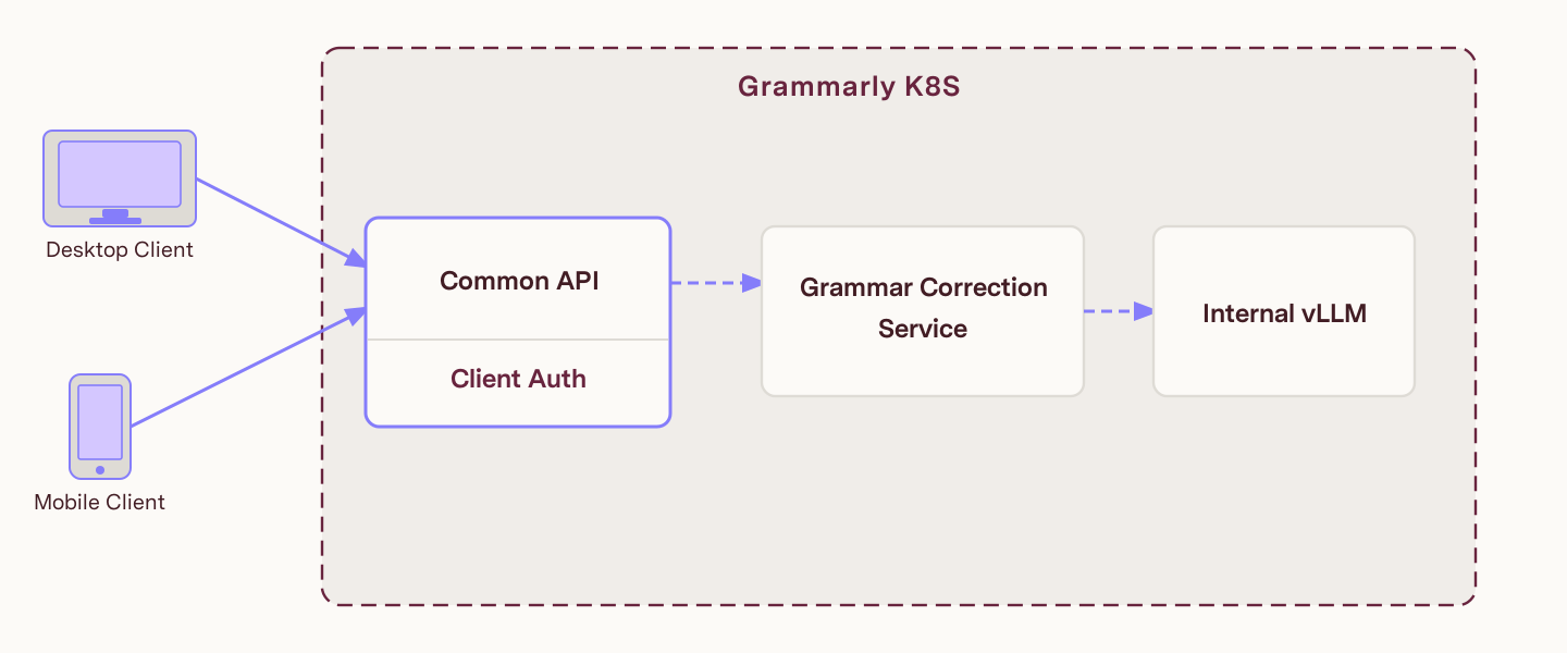
Our original architecture, with a fully internal inference stack

Shifting to external vendors

As our traffic grew, we made a deliberate architectural choice: diversify how and where we run inference so the system stays resilient as we scale. Serving 100 billion requests a week means designing for headroom, redundancy, and flexibility across instance types and regions from the start. We wanted to spend less time on capacity planning, performance tuning, and autoscaling, and more time on model quality and product innovation. An external vendor could help us absorb that operational burden and provide resiliency through multi-region deployments. At the same time, there was a broader strategic desire for a unified data platform that brought data ingestion, processing, and model training and inference into a single system to reduce data siloes and maintenance burdens across teams.  

So we asked ourselves: Could we use a third-party vendor to scale our model serving infrastructure while also making progress toward that unified platform vision?

While the idea had merits, there were real risks. Offloading our serving layer to a managed provider introduced a trade-off: we gained elasticity and resilience, but gave up some direct visibility and control over tuning for a core system. We also didn’t know whether a vendor could meet our performance metrics, especially maintaining real-time latency and high suggestion accuracy while keeping serving costs manageable. 

To find out, we decided to take an experimental approach: we selected one external vendor—Databricks, leveraging their Foundation Model API—and tested it with real production traffic against our internal inference engine to see whether it could meet our requirements.

Evaluating vendor performance

We approached our vendor evaluation performance in three stages: 

1. Validate with shadow traffic: In this phase, we sent duplicate versions of real requests to the third-party system while the internal system served them. This allowed us to conduct an initial validation of the vendor’s stability and scale without disrupting the customer experience. 
2. Harden our LLM gateway/proxy layer: Before we set up an A/B test, we needed a mechanism to authenticate requests and route traffic across providers. Therefore, we had to extend and harden our in-house LLM gateway/proxy layer from ~1,000 RPS to ~100,000 RPS—an increase of almost 100x. 
3. Run an A/B test: Using our internal serving infrastructure as a control, we tested the two vendors on a small percentage of traffic to measure their performance, specifically, latency, suggestion correctness, and cost. 

Running the A/B test

During the experiment, we ran into several challenges, including an upstream, silent image-serving update that briefly degraded output quality, as well as autoscaling edge cases that caused latency spikes. In both cases, our experiment setup allowed us to gracefully shift traffic back to our internal systems while we worked with the Databricks team to debug the issue. Working closely with the Databricks product team, we used these early learnings to refine the platform's autoscaling heuristics and establish robust deployment guardrails, ensuring higher resilience for future rollouts. In many ways, the A/B test became more of a stress test for our working relationship, proving as valuable as the performance data itself. 

With stronger operational guardrails in place, we were able to get a better read on our core performance metrics, except for one: cost. Unlike latency or correctness, cost depends on longer-term traffic patterns, including autoscaling behavior, burst traffic, and idle capacity. To get an accurate comparison, we evaluated cost over a full week of production-like traffic. We compared total weekly cost against the total number of requests and tokens processed to derive a normalized cost per token. We then brought these numbers (along with our internal infrastructure metrics) to Databricks for discussion, which helped us set appropriate cost expectations and push for improvements where needed. 

Rolling out our hybrid infrastructure

As a result of our A/B test, we gained confidence in our hypothesis that using Databricks for GEC inference would help us scale and build resilience. But how much of our serving should we hand off to them? 

We decided on a hybrid approach: relying on Databricks to scale our highest-volume models and our internal infrastructure for highly specialized, experimental, or lower-volume models where we needed additional control and visibility. This approach allows us to leverage the benefits of each system while providing built-in redundancy for the overall system. 

The tradeoff is that we need to manage multiple systems, but that added complexity is worth it because it makes the overall system more resilient. If demand spikes on one system, we can gracefully shift to the other. Plus, through our testing process, we have the operational maturity and vendor relationship to resolve issues quickly when they arise. 

With the hybrid architecture in place, we gradually shifted production traffic to this new system over the following weeks—deliberately monitoring for any regressions before committing the bulk of our traffic. 

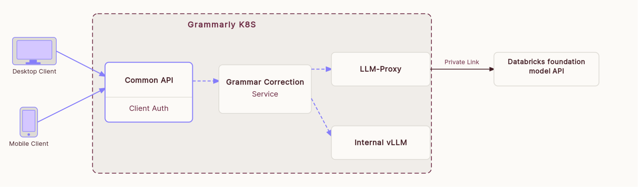
An overview of our hybrid architecture.

Lessons for other teams building production-grade LLM systems

Today, our hybrid GEC-serving infrastructure powers all of our production traffic and sets us up to scale to more customers. Here are some lessons that helped us get here that might help other teams: 

1. Know your use case: Understanding our key requirements helped us confidently evaluate third-party vendors against our internal benchmarks and make the right decision. For us, we needed a vendor that could meet our real-time latency, correctness, and cost benchmarks. These metrics helped us compare the approach and vendor performance. 
2. Don’t assume vendors will be plug-and-play: It’s important to test their solutions against real production traffic to find out if their product works for your use case. These metrics can also serve as leverage in future discussions, allowing you to request performance improvements or negotiate pricing. 
3. Test the team, not just the tech: When assessing vendor performance, technical fixes were only part of the assessment; we also established the right processes and relationships to ensure we got the support we needed when things didn’t go well. This gave us confidence in our working relationship by the time we rolled things out to production. 
4. It can be “both/and”: Traditional vendor conversations are typically approached as a build-or-buy decision. For us, it was useful to do both, as having these systems made our overall architecture more robust.  

— 

If you’re interested in solving infrastructure problems to help people communicate more effectively, come join us. Check out our open roles.