Soft Labels, Hard Wins: Building Better Text Classifiers with LLM Ensembles

By Keith Frazer, Machine Learning Software Engineer, Superhuman
At Superhuman, we’re excited about building AI products that help people think and write more effectively. One way we can do this is by offering suggestions that fit the context of a user’s writing; a personal message, for example, may not need to sound as concise or confident as, say, an email to leadership.
To personalize our suggestions, we need to classify users’ writing into meaningful categories—such as the type of document, task, or audience—to better understand what they are trying to accomplish. However, building these classifiers requires a large swath of labeled data, which we didn’t have. Generating these datasets with human labelers is slow and expensive. Labels generated by large language models (LLMs) are a fast way to create training data, but treating the model’s outputs as hard labels can oversimplify nuanced writing—especially when an example could reasonably fit multiple categories (e.g., an email to ask a friend for a networking chat could be both personal and professional).
Soft-label distillation, on the other hand, can help us better capture these nuances. Instead of assigning a single label, we use a teacher model to produce a probability distribution over all possible labels, thereby better capturing uncertainty in how each example should be classified. Combining multiple teacher models can make that distribution even more reliable. This technique has been fairly well established in machine learning literature, with papers such as Hinton et al. (2015) and Zhou et al. (2021) proving its effectiveness.
But building a pipeline to create these labels, even with frontier models, is less straightforward than it might seem. Frontier models are overconfident by construction; post-training (reinforcement learning from human feedback, or RLHF) is documented to reduce calibration relative to the base model (OpenAI’s GPT-4 report shows exactly this). Our internal analysis confirms this phenomenon, with roughly 99% of raw predictions landing above 0.95 or below 0.05.
To address these challenges, we’ve developed a pipeline to collect soft-label distributions from an ensemble of teacher models, then normalize and aggregate them for student training. In this post, we’ll share our pipeline in more detail, along with tips for other teams on applying this approach to their work.
Choosing our methodology for extracting class probabilities
Before building the pipeline, we had to decide how to extract probability-like scores from the teacher models. Each piece of text required 27 classification outputs across dimensions such as document type (e.g., business or education), writing task (e.g., resume or student essay), and whether it’s a high-stakes task (e.g., an urgent email to your boss). Our goal was to find an approach that could cheaply generate these labels without compromising performance. We evaluated numerous approaches, eventually narrowing it down to two:
- Asking the model to verbalize a confidence score for each label
- Reading the model’s token log probabilities directly for each label
We evaluated both approaches by crafting a prompt for each and comparing the outputs against a sample of anonymized user text. We found that while the verbalizing approach produced a less saturated, softer-looking distribution, its performance was statistically significantly worse than the logprobs approach. This was surprising, as prior work has shown that verbalizing confidence scores can yield better performance than extracting log probabilities for LLMs.
We suspect this gap comes from two things we hadn’t yet invested in: optimizing the verbalized-confidence prompt and (more importantly) having a labeled calibration set to correct the verbalized scores. Given that logprobs were cheap to implement (e.g., no per-model calibration or extra inference calls) and delivered good performance (especially after aggregation and tempering), we decided to move forward with them. That being said, we do think verbalized confidence is a promising direction (and one we hope to revisit in the future).
Building the soft-label pipeline
With our probability extraction approach decided, we could start building our pipeline to create a soft-label distribution, which required us to:
- Create our teacher ensemble with a combination of frontier models
- Extract the probability scores for each teacher model using logprobs and aggregate them
- Apply a domain-knowledge heuristic (in our case, length-dependent temperature scaling) to soften the distribution for student training
Let’s take a closer look at each step.
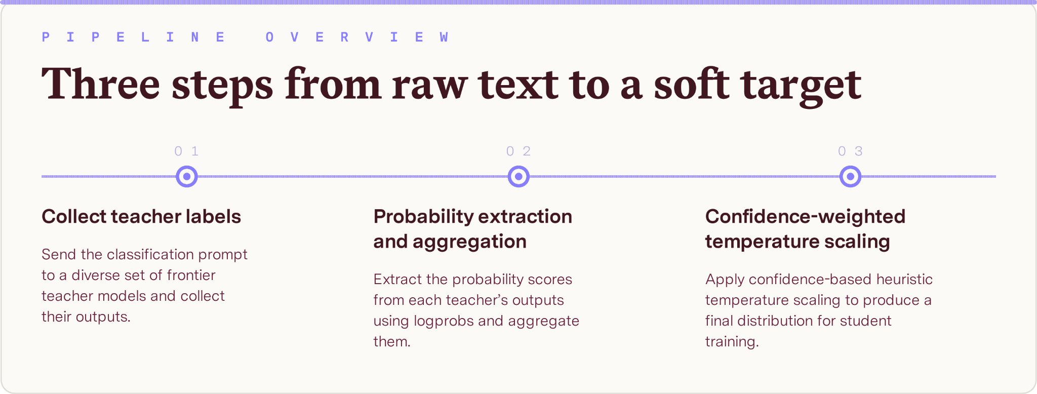
An overview of our soft-label pipeline.
Building the teacher ensemble
To find the right teacher models, we first considered all potential models that our team already had access to: DeepSeek, Claude, GPT, and Gemini. We narrowed this list to models that supported our methodology by returning logprobs in structured JSON output. Structured output simplified the implementation by allowing us to retrieve labels and log probabilities by token index (rather than implementing complex regular expressions).
We ended up with two model families—GPT and Gemini—and decided to use both. The literature is clear that having models from different families increases ensemble diversity, which can better capture uncertainty and improve the quality of soft labels. One trade-off of this approach is that the prompts require some model-specific customization, since each model family has different APIs, ways of defining structured outputs, and minor formatting quirks. We kept the bulk of the prompt the same and made only the minimal required changes, but other teams may find they can improve performance even further by fully customizing each prompt for their respective models.
When selecting the specific models within each family, we initially assumed that choosing the highest-performing models would be best. Our experiments showed, however, that it is important to add a lower-quality, weaker model (like a GPT mini model) to the mix rather than just sticking to the highest-performing models. Raw distributions from the strongest models tend to be sharply peaked—with most labels assigned above 0.98 certainty—leaving little room to model uncertainty. That’s where weaker models come in: They’re more likely to “incorrectly” label some inputs, but those mistakes help us better capture where the real uncertainty lies across the ensemble. This is especially relevant as frontier models get more powerful—research shows they’re increasingly converging, which makes adding weaker models to the ensemble even more valuable.
Calculating the teacher probability scores
With our teacher ensemble chosen, our next step was to extract the probability scores for all class labels for each teacher model.
The first step was to determine whether we should generate all 25 labels at once or prompt the model to produce them individually. To answer this question, we ran an experiment: We prompted one of our teacher models to use each approach on the same 500 texts and then compared the results. We found that the per-label output token probabilities were essentially the same between the two approaches. The only difference was with semantically related labels (like “customer_support_documentation” versus “customer_support_communication”), where seeing all the labels and their definitions at once helped the model better differentiate between them. Therefore, we decided to move forward with asking the model to generate all 25 labels at once.
However, we quickly ran into another challenge when implementing this approach. GPT and Gemini return log probabilities for only a subset of the most likely candidate tokens, many of which are alternate surface forms of the same label, making it impossible to recover probabilities for every class. In fact, we rarely saw more than two of our label tokens in the output. This matters for multiclass classification tasks, as it means we’re always missing some probability mass in the distribution.
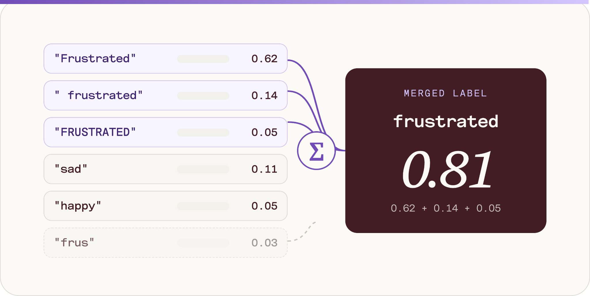
Examples of repeated labels in the model output, which we’ve merged together to create a unified label and probability mass.
To address this, we normalize token variants (e.g., casing and white space differences), aggregate their probabilities into a single label-level probability, and distribute the remaining unseen probability mass across labels not present in the top-k token set.
Once we have probability scores from each teacher, we then combine them into a single number using the arithmetic mean. This helps reduce the impact of any one model’s error or biases on the final distribution.
Producing the final distribution
Even after aggregating the scores, the resulting distributions were still spiky and didn’t capture true uncertainty. Because many models assigned near-100% confidence to their top label, the ensemble output started to resemble a pattern: 100% when all teachers agreed, 83% when one disagreed, 66% when two disagreed, and so on. Diversifying the model family and quality helps introduce uncertainty, but stronger models still dominate the aggregate, masking the contributions of the weaker models. But when should we highlight the contribution of the weaker models more?
Text length immediately jumped out to us. Shorter texts simply contain less information, so they are more likely to produce noisy or ambiguous predictions. After all, a 50-character snippet may be too thin to tell whether a user is drafting a review, a message, a story, or something else entirely. By contrast, longer texts tend to provide enough evidence for the model to make a more reliable distinction. After manually reviewing several examples, we found that this shift seemed to occur around 500 characters.
To turn this intuition into a mathematical adjustment to our labels, we decided to leverage temperature scaling. By dividing the scores by a temperature parameter T, we could smooth the distribution while preserving the class ranking. In other words, the top label stayed at the top, but the probabilities became less extreme. This gave us exactly the behavior we wanted: Examples that already showed meaningful uncertainty became softer, while confident examples were mostly left alone.
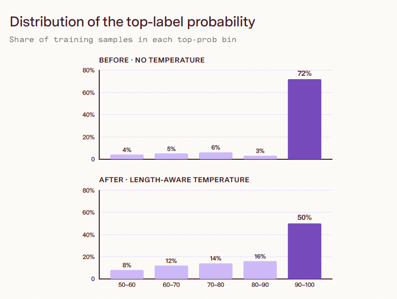
A look at the probability distribution pre- and post-temperature scaling. The final distribution looks less spiky and better reflects the uncertainty in the labels.
Evaluating the effectiveness of our approach
To evaluate this approach, we used this pipeline to generate soft-labeled training data to build three classifiers:
- Register: A multiclass classifier that determines what kind of writing a user is working on (e.g., a fiction story versus an academic research paper)
- High-stakes: A binary classifier that determines if a user is working on a high-stakes or low-stakes writing task (e.g., an email to leadership versus a text to a friend)
- Tasks: A multi-label classifier that determines what task a user is trying to complete with their writing (e.g., writing a school paper versus a sales email)
For each classifier, we compared performance with hard versus soft labels using the area under the precision-recall curve (AUCPR), a standard metric for evaluating a classifier’s performance. Across all three classifiers, soft-label training improved AUCPR by 10% compared with hard-label training. But this raises the question: Did performance improve because the soft-label pipeline produced better top labels or because the student model learned more from the full probability distribution?
To dig into this, we examined the labels from the soft-label pipeline and compared them with the ones from our prior labeling exercise. We found that the soft labels we generated disagreed with the hard labels in only 2% of cases, yet the final performance was much better. We think that for multiclass classifiers, these gains stemmed from the model preserving uncertainty around ambiguous and closely related classes, thereby providing a much richer training signal.
What’s next
This approach has improved the efficiency of generating our training labels, allowing us to iterate more quickly on our classifiers. But we think there’s room for improvement in the technique itself. For instance, what happens if we relax our requirements for model selection (like structured output) to explore other model families? Or revisit the verbalized confidence approach with a calibration dataset?
If you’re excited about helping us answer these questions and other applied ML problems, we’d love to hear from you. Apply to open roles on our Engineering team.